Installation, First Dash App

Ch 01 - Installation

Creating our Solution

Creating our Solution

Welcome to Step 1 of the Beginner’s Guide to Dashboarding!

In order to load and store the data for our dashboard, we must create a new TigerGraph solution.

To do this, we can:

1. Navigate to TigerGraph’s Cloud Portal
2. Login/Register for free using our email address
3. Click on the blue “Create Solution” button
4. Nagvigate to the Healthcare tab
5. Select “Healthcare Engine” Starter Kit

NOTE: For the purposes of learning dashboarding, we will be using TigerGraph’s Healthcare Engine Starter Kit. This Starter Kit comes with over # vertices, # edges, and [still need to finish researching this] data attributes.

   

   

Next, we must enter the details for our solution.

1. Name - This we can simply keep as "Healthcare Engine"
2. Tags - We can add "Dashboard", "Healthcare"
3. Password - By default, it's "tigergraph"
4. Subdomain - This can be "healthcare-dash"

NOTE: Make sure that your subdomain name is unique! (two solutions cannot have the same subdomain at the same time. This subdomain name is used to access your solution (via GraphStudio, for example)

   

   

Once this has been completed, click “Next” and then “Submit”.

And voila, in a few seconds, our solution should go from “Uninitialized” to “Ready”!

Loading our Data

Loading our Data

Ahh, you've reached Step 2 of the Beginner’s Guide to Dashboarding!

Next up, it’s time to load in our data. To do this, we need to:

1. Open GraphStudio by selecting it from the Applications tab
2. Click on MyGraph. This is the graph we’ll be using

NOTE: Additional graphs can be added, deleted, and modified as desired by the user. For the purposes of this dashboard, we will be using the default graph the Healthcare Engine Starter Kit comes with.

   

Time to take a look at our schema! Navigate over to the “Design Schema” tab on the right.

This is our schema, the blueprint of our graph. It consists of vertices connected to one another via edges. Each vertex can be of a different type and contain different attributes. Similarly, edges can be directional, undirected, and even reversed. Each edge can contain different attributes as well, each with multiple datatypes.

Hovering over each component, we see that our schema in this Starter Kit consists of:

   

   

NOTE: This schema can be modified by switching to “Global View” and editing the properties of each vertex and edge. Additionally, vertices and edges may be added and deleted. For a comprehensive guide on creating your own schemas, make sure to check out these resources: TigerGraph Docs, YouTube GSQL 101

Next, we can navigate to the “Map Data to Graph” tab. This section ensures that the raw CSV data files are imported correctly into our graph. Each column is mapped to the appropriate attribute in the appropriate vertex/edge.

In order to modify this mapping, we can simply click the “Edit Data Mapping” icon at the top and select the file and component(s) we wish to map. Next, we click on the source column in the CSV file and match it to the corresponding attribute. When we’re all finished, we can click the “Publish Data Mapping” icon at the top left corner.

   

   

Everything here looks good!

Next up, we can navigate to the “Load Data” tab. Simply press on the white play icon at the top left corner and the loading job should begin automatically. The graph on the right-side displays the progress with respect to time.

When the loading has finished, all CSV files should say “finished”.

Connecting wtih pyTG

Connecting with pyTG

Surprised you made this far, eh? Step 3 of the Beginner’s Guide to Dashboarding!

In order to interface with our Graph, we will utilize pyTigerGraph .

To begin, we can simply install this package by running the following command.

!pip install -q pyTigerGraph

import pyTigerGraph as tg

   

Next, we need to use our solution information from before.

TG_SUBDOMAIN = "healthcare-dash"
TG_HOST = "https://" + TG_SUBDOMAIN + ".i.tgcloud.io" # GraphStudio link

TG_USERNAME = "tigergraph" # This should remain the same...
TG_PASSWORD = "tigergraph"  # Shh, it's our password!
TG_GRAPHNAME = "MyGraph" # The name of the graph

NOTE: As mentioned in the previous document, subdomain names should be unique!

   

Now, we can run the following lines to establish a connection with our solution.

conn = tg.TigerGraphConnection(host=TG_HOST, username=TG_USERNAME, password=TG_PASSWORD, graphname=TG_GRAPHNAME)
conn.apiToken = conn.getToken(conn.createSecret())

print("Connected!")

   

Voila, we’re in!

NOTE: All code segments from this chapter can be found in this Colab Notebook.

Ch 02 - Setting up (First App)

Proper Prerequisites

Proper Prerequisites

While TigerGraph’s Cloud Portal provides the solution, data, and queries needed to analyze our graph, we need the help of another tool to create our dashboard. With Plotly, the task of doing so is made simple, intuitive, and easy.

To begin, we must first install the proper packages.

When running Plotly via a Google Colab, we will first need to use the following command:

!pip install -q jupyter-dash

Jupyter-dash allows the dashboard to be configured for modification via a Python Notebook. This way, the dashboard is updated in real-time with the modification of any cells. Without using the jupyter-dash package, every change made to the dashboard would have to be followed by a recompilation of the app (quite tedious).

Now, we can import our Python libraries with the following line:

import dash
from jupyter_dash import JupyterDash
import dash_html_components as html

The library dash_html_components allows for access to Plotly Dash’s HTML components, allowing us to display HTML elements such as text and linebreaks. We'll cover more of these in the ensuing sections!

Functioning First App

Functioning First App

In order to create our first app, we can simply run the following lines:

app = JupyterDash(__name__)

app.layout = html.Div(children=[
    html.P(children='Hello Dash'),

])

app.run_server(mode='external')

Running the following produces the following output:

Dash App running on:
http://127.0.0.1:8050/

Clicking on the link takes us to our first dashboard!

Great! Albeit, quite simple 😅.

Breaking it down, we can see that our first line initialized the dash app. Since we are running from the Google Colab Notebook, we will use the JupyterDash() constructor instead of the standard app=dash.Dash() constructor.

Next, we define the app’s layout.

Using an HTML .Div() element, we can divide our content into different sections. It is simply a container used to hold other components and establish a structure in our dashboard. For example, our Div element currently contains one element, represented by the attribute children = [...]. Any components contained in the attribute “children” will belong to this html.Div() element. Each children component must be separated by a comma.

   

We can try adding another html.P (a simple paragraph) to our app:

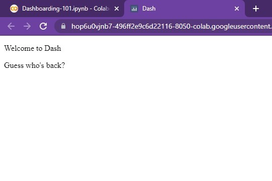
    app.layout = html.Div(children=[
        html.P(children='Hello Dash'),
        html.P(‘Guess who’s back?’),
    ])

Running this will produce the following output to the right:

Ahh, you might have noticed that we’ve omitted the children attribute in the second html.P() statement. This is because ‘children’ is optional and does not to be specified. For example,

   

app.layout = html.Div([
    html.P('Hello Dash'),
    html.P(‘Guess who’s back?’),
])

Running this will produce the following output to the right:

See, same result as above!

NOTE: For more information on .Div(), make sure to check out the following resources: html.Div()

Using Layout Functions

Using Layout Functions

We can create a function to return information to be displayed in our app. This will help make our layout cleaner, more readable, and easier to scale. All content can simply be wrapped in an html.Div() element.

To begin, we can add the following functions and change our layout:

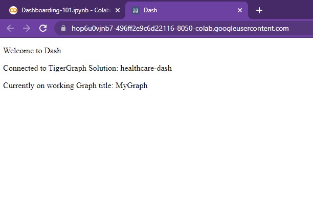
def setup_TG():
  row = html.Div([
              html.P("Connected to TigerGraph Solution Subdomain:", TG_SUBDOMAIN)
              html.P("Currently working on Graph title:", TG_GRAPHNAME)
  ])
  return row


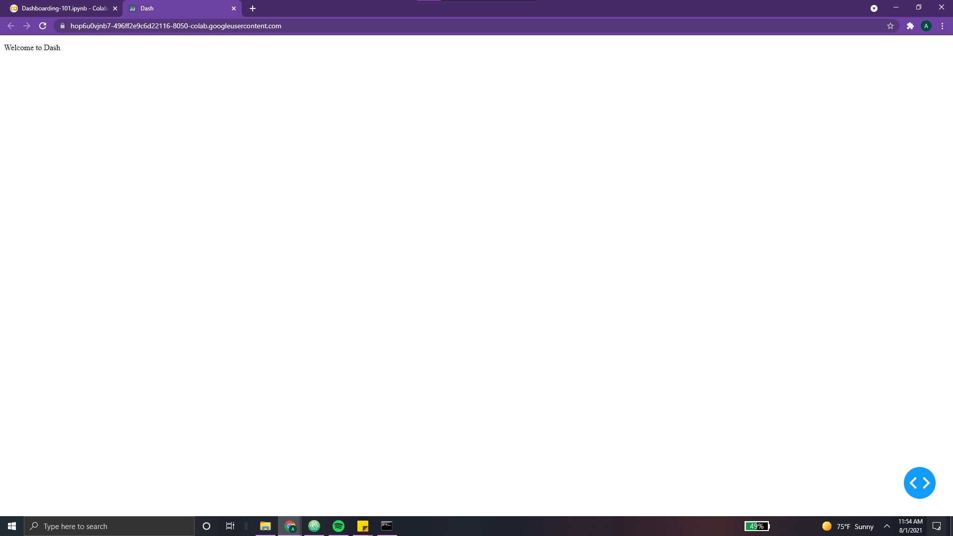
app.layout = html.Div([
    html.P(“Welcome to Dash”)
    setup_TG()
])

And voila, as seen, our app now looks like the following:

These functions can come in quite handy when creating complicated layouts.

Transforming Text

Transforming Text

Dash’s text elements are quite powerful. Here are a few simple ways to spice it up!

We can modify our simple app as follows:

TITLE_STYLE = {
    "background-color": "#abc7ed",
    "margin-bottom": "20px",
    "padding":"5px"
}

def setup_TG():
  row = html.Div([
                  html.P(html.B("Connected to Solution: " + TG_SUBDOMAIN), style={'color':'green'}),
                  html.P(html.I("Currently working on Graph title: " + TG_GRAPHNAME), style={'color':'blue'})
                ])
  return row


app = JupyterDash(__name__)

app.layout = html.Div([
    html.Div(html.H1("Welcome to Dash"), style=TITLE_STYLE), # Adding style, header
    setup_TG() # Adding style, bold, italics
])

app.run_server(mode='external')

Here's the resulting output:

Let's break it down, component by component!

   

HTML Headers

One of the easiest ways to spice up one's dashboard is to vary the text styles. This can be done using simple HTML header elements (H1, H2, H3, H4, H5, H6). A table showing each one's output can be found below.

Header 1	Headers 4 - 6	Header 3	Header 4	Header 5	Header 6
What's Up?	Good Day.	Bless You!	Well done.	Happy Birthday!	Goodbye?

The specific style of each will change based on the font. However, the relative sizes can be seen above.

NOTE: For more information on HTML, feel free to check out the following resources: Dash Headers, Dash HTML

   

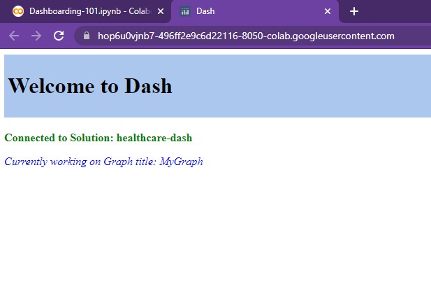
In line 18 of our code snippet, we see that our html.P() element is now html.H1().

    html.Div(html.H1("Welcome to Dash"), style=TITLE_STYLE), # Adding style, header

Pretty simple and effective! Ahh, you may have noticed the html.Div() element that the header is wrapped in. Let's take a closer look at the reason for this...

   

Style Dictionary

One of the best ways to style a dashboard is to use a style dictionary. In these dictionaries, one can specify attributes such as background color, padding, margins, font style, font color, etc.

In lines 1- 5, we explicitly create a style dictionary titled TITLE_STYLE.

TITLE_STYLE = {
    "background-color": "#abc7ed",
    "margin-bottom": "20px",
    "padding":"5px"
}

This dictionary is then passed into the html.Div() element which contains our header. As a result, the header is given extra padding, margin, and a light-blue background. Pretty straightforward!

This style dictionary doesn't have to be stored in a variable.

In lines 9 and 10, we explicitly change the colors of each html.P() using the keyword style.

html.P(html.B("Connected to Solution: " + TG_SUBDOMAIN), style={'color':'green'}),
html.P(html.I("Currently working on Graph title: " + TG_GRAPHNAME), style={'color':'blue'})

NOTE: Color can take both keywords (ex. common colors like red, orange) as well as hex values (ex. 'DD659F')

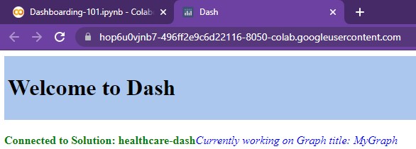
This brings us to our next point, the html.B() and html.I() used in lines 9 and 10.

   

Html.B(), Html.I()

In order to bold or italicize sections of text, we can simply use html.B() and html.I()

These elements can stand on their own without being wrapped in html.P() elements. However, this removes the division between two lines. For example, the following two lines produce the following output:

html.B("Connected to Solution: " + TG_SUBDOMAIN, style={'color':'green'}),
html.I("Currently working on Graph title: " + TG_GRAPHNAME, style={'color':'blue'})

NOTE: For more information on these two elements, feel free to check out the following: html.B(), html.I()

   

There are so many more ways to transform text! We'll cover other methods in Chapter 05 - Sheriff Styles!

NOTE: All code segments from this chapter can be found in this Colab Notebook.